The power of Central Limit Theorem is widely known. In the following post we are exploring a bit the areas outside its scope – where the CLT does not work. We present the results of numerical simulations for three distributions: Uniform, Cauchy distribution, and certain “naughty” distribution called later “Petersburg distribution”.

The CLT is formulated in a various ways. We will use the following simplified formulation:

For any distribution \(x\) having finite expected value \(\mu_x\) and variance \(\sigma_{x}^{2}\), the new variable made of:

$$y = \frac{1}{n} \sum_{i=1}^{n} x_i$$

tends to Gaussian distribution as n increases, and has the parameters:

$$\mu_y = \mu_x,$$
$$\sigma_y = \frac{\sigma_x}{\sqrt{n}}$$

What a delighting theorem! Whatever \(x\) distribution we have, the distribution of its averages tends to Gaussian. Works for any \(x\) distribution. Well… almost any distribution. The initial distribution should have finite expected value and variance. We usually leave this fact with the comment: “works for all properly behaving distributions”. Lets check what is the result for “improperly behaving” distributions.

The main actors in our show are as follows:

• Cauchy distribution – often called Breit-Wigner distribution in the world of physics. It has infinite variance and mean in spite of looking very innocent.
• “Petersburg distribution”, comes from so called St. Petersburg Paradox. Like in the previous case: \(\mu\) is infinite, as well as \(\sigma^2\). Its amusing that a rather innocent game (see Wikipedia’s article) leads to such distribution.
• Uniform distribution – nothing unusual, well defined \(\mu\) and \(\sigma^2\) used just for reference

The samples are generated using Mersenne Twister pseudo-random numbers generator. The “Petersburg” series are generated using the following code:

    
def single_petersburg_game():
    sum_won = 0
    n = 1
    while True:
        d = random.random()
        if d > 0.5:
            sum_won = n
            n *= 2
        else:
            break

    return sum_won
    

The numerical experiments were done by drawing \(10^9\) pseudo-random numbers having given distribution. Then for sampling distribution we used \(10^5\) samples, each of size \(100\).

Lets start with the most common case – uniform distribution. As we see on the figure below, nothing surprising is here:

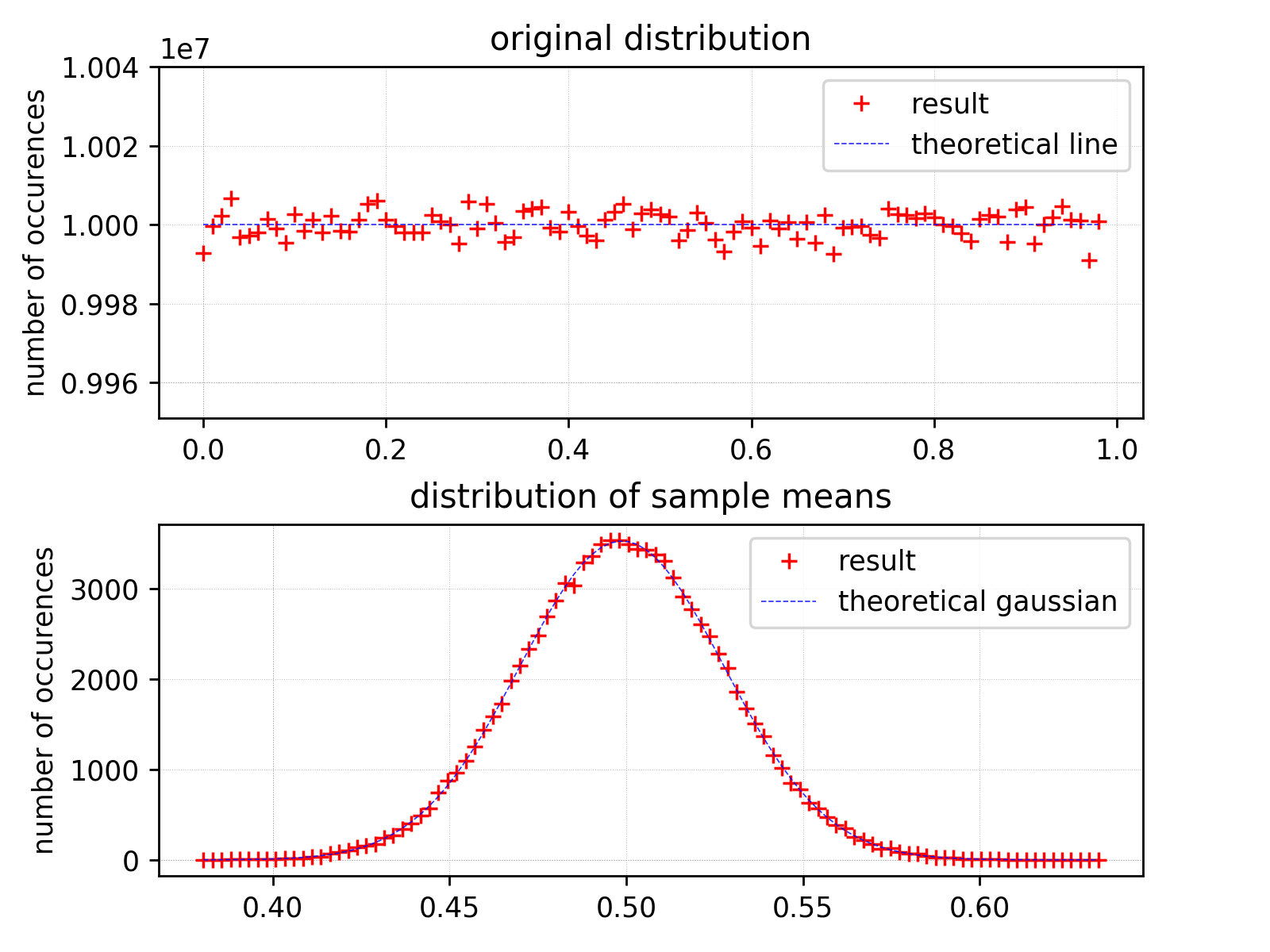
The top chart shows the original distribution, the bottom one distribution of sample means. As we expected, we observe nice Gaussian here. As we see, CLT works great and the most interesting part is still ahead.

Now have a look at the analogous histograms produced for Cauchy distribution (please note the logarithmic scale on y axis):

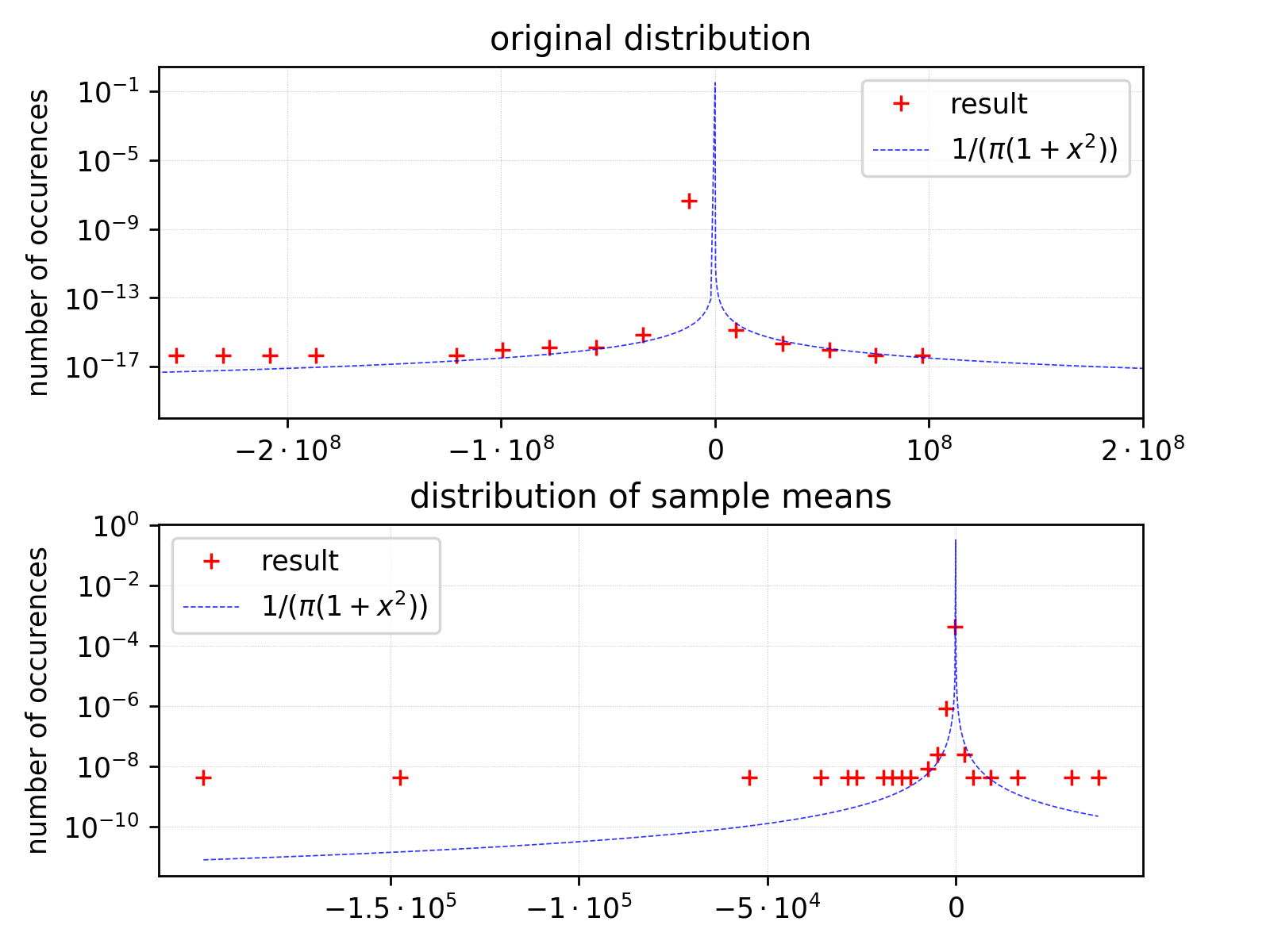
The situation is significantly different here. The population size, sample size and the number of samples are the same as in previous example. The only difference is an input distribution.
I does not require any statistical tests to state that the distribution of sample means (SM) is far from being gaussian one. The maximum for SM distribution has the sample position as for
the original distribution. However the area beyond is definitely standing out (please note the range being much shorter on x axis than for population distribution, which is characteristic of SM distributions).
So – not Gauss and not longer Cauchy. Thus we observe the situation outside the scope of central limit theorem.

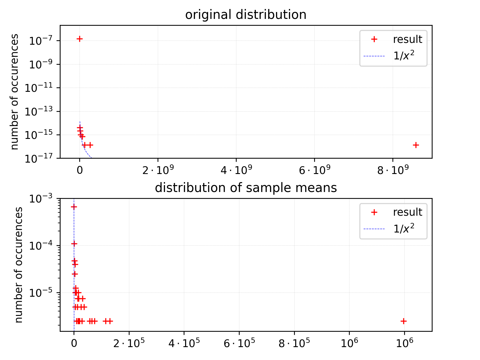
And now the most interesting part: “Petersburg” distribution – having infinite variance and expected value. Lets see how it looks like (double logarithmic scale):

We use the same population/sample sizes as before, the scale on y axis is logarithmic. We plot \(y=1/x^2\) together with distribution points in order to have an idea how the distribution roughly looks like).
One can also see x-log scale plot which gives us another look on the distribution of sample means. We can observe that values moved to the right from the reference \(1/x^2\) curve for distribution of sample means. As for now it looks that we can not expect observing any other tendency for this distribution.

At the end we would like to summarize this post with the following:

Do not trust the distributions with infinite variance and expected value 😉

In the next part we will consider the behaviour of standard deviation for presented distributions.

Mikołaj Sitarz, 2018