In the following article, we will look at image recognition using linear regression. We realize that this idea may seem quite unusual. However, we will show using a simple example, that for a certain class of images, and under quite strictly defined circumstances, the linear regression method can achieve surprisingly fair results.
Description
At the very beginning, we would like to reassure our readers – we will not convince anyone to abandon convolutional neural networks in favor of linear regression. The presented method will only allow us to gain better insight into the simple image recognition process itself.
For our purposes, we will use the Fashion MNIST collection, published by Zalando (available on github). This is a collection of 70,000 images containing different pieces of clothing such as T-shirt, pants, shoes, tracksuits, etc. (each category has been assigned a numerical value: 0 – T-shirt, 1 – pants, 2 – pullover, …). Each is a grayscale image with a size of 28×28 pixels.
![]()
Trivial case – images composed of a single pixel
Before we move on to the actual image recognition algorithm, let us consider a trivial example – a picture containing one grayscale pixel, with values from 0 to 255. For each “picture” in such a set, we assign a value of -1 or 1 (e.g.: -1 is “night” and 1 is “day”). The hypothetical set contains the classified “pictures” with -1/1 values assigned to them. This set will be used first, to present the classification method itself. In this case, we will apply the classical linear least squares algorithm and fit a straight line to the given set, as presented in the illustrative figure below:
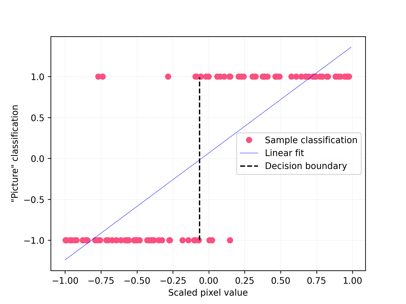
For more convenient calculations, the values on the x-axis from 0 to 255 have been scaled to the interval (-1, 1). The individual points in the graph represent individual single-pixel “pictures”. Formally, here we are looking for the parameters \(a\) and \(b\) for a straight line with equation:
$$ y = a x + b $$
where \(x, y \in \mathbb{R}\), by minimizing the sum of squares of the distances of all points from the line. For a straight line fitted in this way, we consider the test sample to have a value of “1” when the calculated \(y > 0\), otherwise “-1”. That gives us the decision boundary as a vertical straight line crossing the point where the fitted line intersects the \(x\) axis.
Thus, the two classes of “pictures” are separated simply by a straight line, capturing the decision boundary for the set so defined quite well.
T-shirt recognition for 28×28 pixels images
So far, the method is trivial. We must admit however, that such an application of linear regression is not very practical, we are unlikely to use single-pixel images daily. So, we will extend the method to work for real images. Let us return to the actual task and the MNIST fashion set. For each of the images, we will retrieve the numerical values assigned to each pixel:
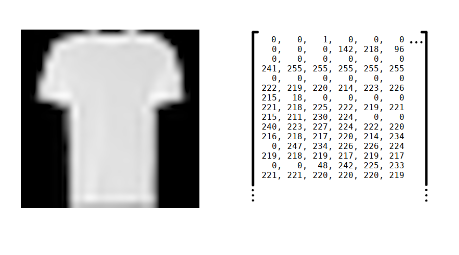
From the matrix thus formed, we will form a vector by concatenating successive rows of it. So, each 28×28 pixel image, will be represented by a 784-dimensional vector of real numbers. As in the previous case, we want to create a binary classifier – that is, one that gives us a “yes” or “no” answer (1, -1). This time, we want to recognize whether there is a t-shirt (1) or another piece of clothing (-1) in the given picture. So, we are now looking for 785 \(\theta\) parameters describing a 784-dimensional hyperplane:
$$y = \theta_0 + \sum_{i=1}^{784} \theta_i x_i$$
We will not publish a graphic representation of the 784-dimensional hyperplane, due to some technical limitations of our software.
Let us denote now the value of \(y\) calculated for a single sample \(i\) according to the above formula, as \(\hat{y}^{(i)}\) and the actual value as \(y^{(i)}\). The optimization objective will be the loss function, defined as:
$$\mathrm{L}(\theta) = \sum_{i=1}^{m} \left(y^{(i)} – \hat{y}^{(i)} \right)^2$$
where \(m\) is the number of images in the set under study. The goal is to find \(\theta\) parameters for which \(\mathrm{L}\) reaches minimum – classic least squares method, nothing more.
The authors of the Fashion MNIST collection recommend that 60000 images be treated as a training set and 10000 as a test set. To simplify the considerations, we will create new sets that consist of 50% images showing “t-shirt” and 50% images with other clothes. After this procedure, our training set contains 12000 images, and the test set contains 2000 of them.
Pixel values between 0 and 255 will be normalized using convenient scikit-learn normalizer. We will classify the result as positive “1” (t-shirt) if the calculated \(y\) value is greater than zero. Otherwise, we will consider the result as a negative “-1” (any other garment).
The quality of the classifier, we will measure with the commonly used parameter – accuracy, defined as:
$$A = \frac{\mathrm{TP} + \mathrm {TN}}{\mathrm{TP} + \mathrm{TN} + \mathrm{FP} + \mathrm{FN}}$$
Where subsequent quantities are represented as: \(\mathrm{TP}\) – true positives, \(\mathrm{TN}\) – true negatives, \(\mathrm{FP}\) – false positives, \(\mathrm{FN}\) – false negatives.
Result
Following the commonly accepted methodology, the hyperplane parameters were fitted using the training set, while the classifier quality was evaluated on the test set. Since both sets contain half of the “positive” images (t-shirts) – the lower bound here will be a random classifier (randomizing the result with probability ½), which would give us an accuracy of 50%.
And here is the result obtained for the linear regression classifier – accuracy parameter for the test set:
$$A_{\%} = 92.5\%$$
When we consider that this machine learning method is one of the simplest, this is an unexpectedly satisfactory result (94.9% on the training set). The following table provides a detailed summary of the experiment:
| Overpredicted samples | 89/2000 (4.45%) |
| Underpredicted samples | 61/2000 (3.05%) |
| Accuracy | 92.5% |
| F1 | 92.6% |
Summary
The achieved result suggests that a significant part of the used set is linearly separable. Such circumstances as strictly narrowed set of images, their small size and appropriate choice of distribution of both sets also contributed to the final favorable result.
As the number of dimensions increases, classical linear regression gains quite interesting possibilities and applications.
The source code used for the calculations: cv_linreg.py
Mikołaj Sitarz, 2021
![]()